Bayesian Approach to Ranking Movies

Many people like watching movies, and I do too. Recently I've discovered this somewhat sketchy Korean site that hosts quite a few movies online. I call it sketchy because I almost always see ads asking me to download a piece of software that's supposed to protect my computer from a deadly virus whenever I click on just about anything. Nonetheless, my goal is to watch a movie online, and so far the site has never failed to let me down.

Here is an example page with a thumbnail image for each movie along with its total number of upvotes, downvotes, and views received since the first upload. The site allows you to sort the movies based on the upvotes, views, or upload dates. I'm going to scrape all such pages and use the information about movies to efficiently rank them using a Bayesian procedure.

Below is a full working R script to grab movie titles and the associated upvotes, downvotes, views, and image urls. Make sure to set .parallel = FALSE when running the loop for the first time and let it run for few iterations. Then set .parallel = TRUE and run it again fully. I used the rvest library to make my web scraping easier and more robust. The code runs in about a minute using a single physical CPU with 8 cores on a Mac. If you are using a Windows, then you might want to use doSNOW or doParallel instead of doMC. Use detectCores() function to check how many cores your laptop has available.

library(plyr)
library(data.table)
library(rvest)
library(doMC)
library(ggplot2)

registerDoMC(8)
base_url <- "http://nojehu.com/bbs/board.php?bo_table=streaming05&page="
page_end <- 500
starttime <- Sys.time()
dat <- llply(1:page_end, function(i) {
  movies <- read_html(paste0(base_url, i))
  titles <- movies %>% 
    html_nodes(".gall_text_href") %>%
    html_text() %>% 
    gsub("댓글[0-9]+개", "", .) %>%
    gsub("\\s+", "", .)
  upvotes <- movies %>% 
    html_nodes(".gall_con li:nth-child(4) strong") %>%
    html_text()
  downvotes <- movies %>%
    html_nodes(".gall_con li:nth-child(5) strong") %>%
    html_text()
  views <- movies %>%
    html_nodes(".gall_text_href+ li") %>%
    html_text() %>%
    gsub(".*([0-9]+)$", "\\1", .)
  image_urls <- movies %>%
    html_nodes(".gall_href img") %>%
    html_attr("src")
  output <- data.table(cbind(titles, upvotes, downvotes, views, image_urls))
  cat(paste0("Page ", i, "scraped!\n"))
  return(output)
}, .parallel = TRUE)
print(Sys.time() - starttime)

f <- rbindlist(dat, fill = TRUE)
cols <- c('upvotes', 'downvotes', 'views')
f[, (cols) := lapply(.SD, as.numeric), .SDcols = cols]

Now that I have the data, let's use the number of upvotes, downvotes, and views to rank movies efficiently. When it comes to ranking movies using upvotes and downvotes, we are inherently dealing with positive and negative observations where an upvote corresponds to a success and a downvotes a failure. In statistics, we model such set of binary data using a binomial distribution. In Bayesian setting, we'd use a beta prior with a binomial likelihood to construct a beta posterior.

Here's what I mean. The maximum likelihood estimate of the true proportion of upvotes of a movie is the total number of upvotes divided by the total number of votes for that movie. However, this estimate, while intuitive and uncomplicated, is not so reliable when we have new movies with zero or small number upvotes. In that case, Bayesians tend to make use of prior information by borrowing data from the whole - that is, the proportion of total upvotes and downvotes of all movies. These global proportion of upvotes and downvotes serve as prior pseudo counts, and we add them to our actual data - the number of upvotes and downvotes of each movie - to get the parameter estimates of a beta posterior. Then instead of using the posterior mean or mode, I use the 10th quantile of a beta posterior as a measure of rank. The greater the score, the higher the rank of a movie.

upvote_total <- sum(f$upvotes)
downvote_total <- sum(f$downvotes)
f[, totalvotes := upvotes + downvotes]
f[, rank_naive := qbeta(0.1, 10*upvote_total/(upvote_total + downvote_total) + upvotes, 10*(1 - upvote_total/(upvote_total + downvote_total)) + downvotes)]

As you see, this naive Bayesian rank score doesn't take into account the vote popularity of each movie. The vote popularity of a movie can be approximated as the total number of upvotes that the movie has received divided by the votes total across all movies. Below I added popularity proportions as another set of pseudo counts for a beta posterior. Note that I multiplied the popularity proportions by 10 to give them more weight.

f[, rank_popular := qbeta(0.1, 10*upvote_total/(upvote_total + downvote_total) + 10*totalvotes/sum(totalvotes) + upvotes, 10*(1 - upvote_total/(upvote_total + downvote_total)) + 10*(1- totalvotes/sum(totalvotes)) + downvotes)]

But again, even this popularity Bayesian rank score fails to incorporate the view popularity of a movie. The view popularity of a movie is calculated as the total number of views the movie has received over the views total across all movies.

f[, rank_agg := qbeta(0.1, 10*upvote_total/(upvote_total + downvote_total) + 10*totalvotes/sum(totalvotes) + 10*views/sum(views) + upvotes, 10*(1 - upvote_total/(upvote_total + downvote_total)) + 10*(1- totalvotes/sum(totalvotes)) + 10*(1 - views/sum(views)) + downvotes)]

I have three types of rank scores, each successively adding more information independently. Let's plot the scores by rank and compare the three approaches.

f1 <- f[order(-rank_naive)]
f2 <- f[order(-rank_popular)]
f3 <- f[order(-rank_agg)]

f1[, Type := "Naive Rank"]
f2[, Type := "Popularity Rank"]
f3[, Type := "Aggregate Rank"]
total <- rbind(f1[, .(Type, Rank = 1:nrow(f), Score = rank_naive)], 
               f2[, .(Type, Rank = 1:nrow(f), Score = rank_popular)],
               f3[, .(Type, Rank = 1:nrow(f), Score = rank_agg)])
g <- ggplot(total, aes(x = Rank, y = Score, colour = Type)) + 
  geom_point() +
  theme(legend.position = c(0.8, 0.8), legend.background = element_rect(size = 0.5, linetype = "dotted")) + 
  ggtitle("Comparison of Different Types of Bayesian Ranking")
plot(g)

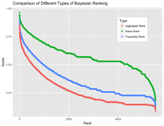
As I add more information as prior, the curve becomes smoother. This means that there are fewer flat lines where movies can have same rank scores. Eventually the curve is expected to look like a reciprocal function as more information is added as pseudo counts. For example, we can further use an exponential decay function to take into account the upload date of each movie in order to distinguish scores among movies that are uploaded on the same day. We can also add information about the overall popularity of movies in other sites such as Netflix and IMDB or adjust the weights of each pseudo prior counts.

Here are the top 5 movies for each type of ranking methods:

• Naive Rank

• Popularity Rank

• Aggregate Rank

Whether this kind of shuffle in rank is effective in recommending which movies to watch I am not sure. We need to measure the performance of each type of rank through A/B testing and then compute precision and recall of which of the movies recommended as top-k are actually clicked or seen.

The drawback of this Bayesian approach to ranking is that the prior informations are added independently. Some information may be correlated with others, and this may be something that needs to be addressed. However, the beauty of this technique lies in efficiency and simplicity.