Bayesian Zero-Inflated Poisson Model
Posted on July 05 2017 in Bayesian Statistics
Wikipedia defines
The zero-inflated Poisson model concerns a random event containing excess zero-count data in unit time. For instance, the number of insurance claims within a population for a certain type of risk would be zero-inflated by those people who have not taken out insurance against the risk and thus are unable to claim.
Specifically, the model can be broken down into two components that correspond to two different zero generating processes. The first is under a binary distribution that generates structural zeroes, and the second process is subject to a Poisson distribution that generates counts, some of which may be zero.
The two model components are aggregated as follows:
Suppose \(Y_1, ..., Y_n | \theta, \lambda \sim P(Y = y | \theta, \lambda)\) (iid) where
where \(y = 0, 1, 2, ...\), \(\theta \in [0,1]\), and \(\lambda > 0\). Typically, \(\theta\) and \(\lambda\) are assumed to be unknown constants, meaning their values are fixed; however, Bayesians assign a prior distribution to an unknown variable which makes possible making inference on it using Bayes rule.
Suppose the priors are specified as \(\theta \sim Beta(a,b)\) and \(\lambda \sim Gamma(c,d)\) where \(a, b, c, d\) are fixed hyperparameters.
obs <- scan("ZIP.txt")
hist(obs, main = "Histogram of 1000 observations", xlab = "Observations")
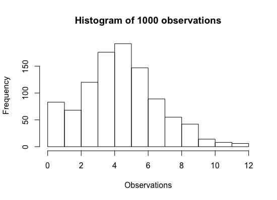
The synthetic dataset contains 1000 observations from the model specified. Generate samples from the posterior distribution of interest \(f(\theta, \lambda | y_1, ..., y_n)\) with Markov chain Monte Carlo (MCMC) simulation. I'm going to use three chains with overdispersed initial values (with respect to the true marginal posterior distributions) for \(\theta\) and \(\lambda\) in each chain.
set.seed(28473)

# function to convert theta to psi
# theta between 0 and 1
# psi is real-valued
conv_theta <- function(theta) {
  return(log(theta/(1-theta)))
}

# function to convert psi to theta
conv_psi <- function(psi) {
  return(exp(psi)/(1+exp(psi)))
}

# function to calculate h(theta)
log_theta_h <- function(theta, lambda) {
  return(nA*log((theta+(1-theta)*exp(-lambda))) + (a-1)*log(theta) + (nB+b-1)*log(1-theta))
}

# function to calculate h(lambda)
log_lambda_h <- function(lambda, theta) {
  return(nA*log((theta+(1-theta)*exp(-lambda))) - nB*lambda - d*lambda + (syB+c-1)*log(lambda))
}

# set hyperparameters to make priors uninformative
a <- b <- 1
c <- d <- 0.01

# set data values
nA <- sum(obs == 0)
nB <- sum(obs > 0)
syB <- sum(obs[obs > 0])

# set mcmc parameters
mcmc_samples <- 20000
chains <- 3
metrop_var <- 0.3
accept_theta <- accept_lambda <- rep(1, times = chains)

# create matrices to store posterior theta and lambda values
theta <- lambda <- matrix(0, nrow = mcmc_samples, ncol = chains)

# set overdispersed initial values of theta and lambda
theta[1,] <- c(0.1, 0.8, 0.9)
lambda[1,] <- c(10, 20, 100)

for (i in 2:mcmc_samples) {
  theta[i,] <- theta[(i-1),]
  lambda[i,] <- lambda[(i-1),]

  theta_proposed <- conv_psi(rnorm(n = chains,
                                   mean = conv_theta(theta[(i-1),]),
                                   sd = sqrt(metrop_var)))
  ratio_ht <- exp(log_theta_h(theta_proposed, lambda[(i-1),]) -
                    log_theta_h(theta[(i-1),], lambda[(i-1),]))
  for (j in 1:chains) {
    if (ratio_ht[j] >= runif(n = 1, min = 0, max = 1)) {
      theta[i,j] <- theta_proposed[j]
      accept_theta[j] <- accept_theta[j] + 1
    }
  }

  # update lambda
  lambda_proposed <- rnorm(n = chains,
                           mean = lambda[(i-1),],
                           sd = sqrt(metrop_var))
  for (j in 1:chains) {
    if (lambda_proposed[j] > 0) {
      ratio_lt <- exp(log_lambda_h(lambda_proposed[j], theta[i,j]) -
                        log_lambda_h(lambda[(i-1),j], theta[i,j]))
      if (ratio_lt >= runif(n = 1, min = 0, max = 1)) {
        lambda[i,j] <- lambda_proposed[j]
        accept_lambda[j] <- accept_lambda[j] + 1
      }
    }
  }
}

atable <- rbind(accept_theta/mcmc_samples, accept_lambda/mcmc_samples)
dimnames(atable) <- list(c('theta', 'lambda'), c('chain 1', 'chain 2', 'chain 3'))
print(atable)
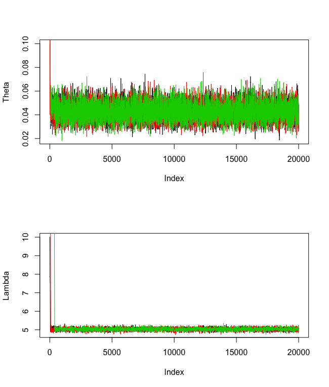
There is evidence to suggest that the chains have converged since the traceplots look converged after roughly about 2000 iterations. Let's set the burn-in amount to 2000.
library(coda)

# trace plots
# theta looks good
# lambda looks permissible
par(mfrow = c(2,1))
plot(theta[,1], type = "l", ylab = "Theta")
for (j in 2:chains) {
  lines(theta[,j], col = j)
}

plot(lambda[,1], type = "l", ylab = "Lambda")
for (j in 2:chains) {
  lines(lambda[,j], col = j)
}
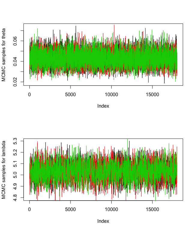
Below are the traceplots after removing the first 2000 burn-in samples:
# burn-in amount: 2000 chosen by looking at the trace plots
burnin <- 2000
plot(theta[(burnin+1):mcmc_samples,1], type = "l", ylab = "MCMC samples for theta")
for (j in 2:chains) {
  lines(theta[(burnin+1):mcmc_samples,j], col = j)
}
plot(lambda[(burnin+1):mcmc_samples], type = "l", ylab = "MCMC samples for lambda")
for (j in 2:chains) {
  lines(lambda[(burnin+1):mcmc_samples,j], col = j)
}
The autocorrelation plots (not shown) look good since the lags decay quickly. The effective sample sizes seem permissible so there are enough posterior samples to make proper inference. Gelman and Rubin diagnostics are all less than 1.1 which is a good sign.
# autocorrelation plots look good
# lags decay quickly
par(mfrow = c(3,2))
for (j in 1:chains) {
  acf(theta[(burnin+1):mcmc_samples,j])
  acf(lambda[(burnin+1):mcmc_samples,j])
}

# effective sample sizes are permissible
ess_theta <- ess_lambda <- rep(0, times = chains)
for (j in 1:chains) {
  ess_theta[j] <- effectiveSize(theta[(burnin+1):mcmc_samples,j])
  ess_lambda[j] <- effectiveSize(lambda[(burnin+1):mcmc_samples,j])
}
etable <- rbind(ess_theta, ess_lambda)
dimnames(etable) <- list(c('ESS theta', 'ESS lambda'),
                         c('Chain 1', 'Chain 2', 'Chain 3'))
print(etable)

# Geweke diagnostics
gew_theta <- gew_lambda <- rep(0, times = chains)
for (j in 1:chains) {
  gew_theta[j] <- round(geweke.diag(theta[(burnin+1):mcmc_samples,j])[[1]], 3)
  gew_lambda[j] <- round(geweke.diag(lambda[(burnin+1):mcmc_samples,j])[[1]], 3)
}
gtable <- rbind(gew_theta, gew_lambda)
dimnames(gtable) <- list(c('Geweke theta', 'Geweke lambda'),
                         c('Chain 1', 'Chain 2', 'Chain 3'))
print(gtable)

# Gelman and Rubin diagnostics
# all less than 1.1 which is a good sign
total_count <- mcmc_samples - burnin
keep_set1 <- seq((burnin+1), burnin+(total_count/2), 1)
keep_set2 <- seq(burnin+(total_count/2)+1, mcmc_samples, 1)

mh.list1 <- list(as.mcmc(theta[keep_set1, 1]),
                 as.mcmc(theta[keep_set2, 1]),
                 as.mcmc(theta[keep_set1, 2]),
                 as.mcmc(theta[keep_set2, 2]),
                 as.mcmc(theta[keep_set1, 3]),
                 as.mcmc(theta[keep_set2, 3]))
mh.list1t <- mcmc.list(mh.list1)
print(gelman.diag(mh.list1t)$psrf)

mh.list2 <- list(as.mcmc(lambda[keep_set1, 1]),
                 as.mcmc(lambda[keep_set2, 1]),
                 as.mcmc(lambda[keep_set1, 2]),
                 as.mcmc(lambda[keep_set2, 2]),
                 as.mcmc(lambda[keep_set1, 3]),
                 as.mcmc(lambda[keep_set2, 3]))
mh.list2l <- mcmc.list(mh.list2)
print(gelman.diag(mh.list2l)$psrf)
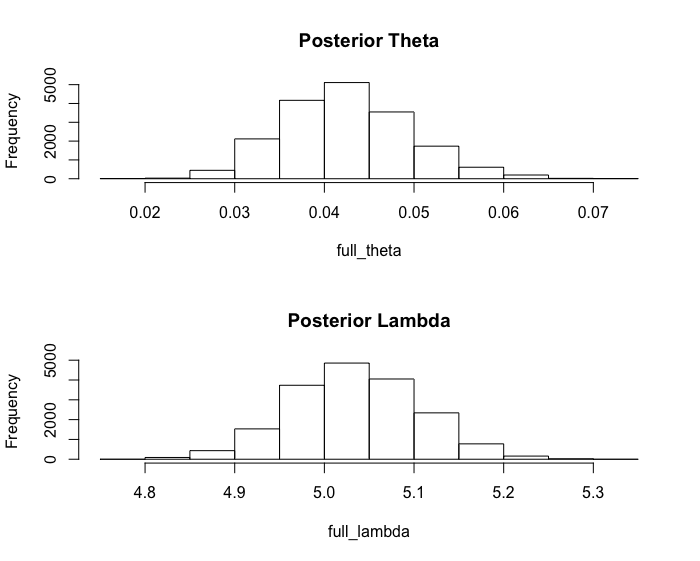
The posterior mean of \(\theta\) is 0.0424 and that of \(\lambda\) is 5.034. The posterior standard deviation of \(\theta\) is 0.007024 and that of \(\lambda\) is 0.07197. The 95% quantile-based, equal tail credible interval estimate for \(\theta\) is (0.0298, 0.0573) and that for \(\lambda\) is (4.894, 5.172).
# final inference for theta and lambda
full_theta <- theta[(burnin+1):mcmc_samples]
hist(full_theta)
quantile(full_theta, c(0.025, 0.975))
mean(full_theta)
sd(full_theta)

full_lambda <- lambda[(burnin+1):mcmc_samples]
hist(full_lambda)
quantile(full_lambda, c(0.025, 0.975))
mean(full_lambda)
sd(full_lambda)