Estimating the Total Daily Number of Customers at Bon Me

Bon Me is one of my favorite places to grab a quick bite for lunch. Surprisingly I didn't know about its existence until earlier last year despite being so close to my workplace. I really recommend you try miso-braised pulled pork on brown rice without cilantro. It's really addicting.

Anyhow, when you order food at Bon Me, you are given a receipt with a number that represents your order number. For example, if I get a receipt that had number 20 on it, it means that I'm the 20th customer of the day and there are 19 people who already ordered food before me. Simply said, each receipt, likewise a customer who holds it, is numbered in sequence. Then would it be possible to estimate the total number of customers Bon Me serves on a given day using a sample of those numbered receipts? Let's simplify the problem by assuming we have a pile of receipts in a box at the end of the day and decide to sample five receipts without replacement independently and randomly from the pile. The receipt numbers are ordered like below:

Intuitively, a naive practitioner of statistics would say the total number of people at Bon Me on this day is 250 based on this five number sample. But is it really 250? Clearly there is a chance the total number of customers is greater than 250 since what we are looking at is only a sample. We don't know the exact total number of receipts/customers (since that's what we are trying to estimate duh!), but the fact we have four numbers 6, 18, 20, 99 below 250 means it's not at all unlikely we will see numbers higher than 250 either. The Bayesians would remedy this problem by putting a distribution around that number to quantify their uncertainty with the estimate. I can show you how to mathematically derive the formula using combinatorics and the laws of probability, but the focus of this blog post is to estimate the total number of customers at Bon Me on a given day by constructing a hierarchical Bayesian model in R with JAGS. JAGS, as I mentioned in the earlier post, is a software which stands for Just Another Gibbs Sampler that runs complex MCMC simulations from a generative model. Instead of JAGS, you can also use BUGS or Stan; though I like Stan more, JAGS should work fine in many situations.

the problem set-up

Let's say the total number of receipts from Bon Me on a given day is \(K\). Of those \(K\), let's call the five number sample above we happen to observe as data \(D\). Then we want to know the posterior probability of the number of receipts \(K\), given data \(D\) on which receipt numbers have been observed so far:

where \(P(D | K)\) refers to the likelihood of observing all the receipt numbers given the actual number of receipts in existence \(K\) which I assume to be discrete uniformly distributed with the minimum at \(0\) and the maximum at \(K\). When deciding which distribution to use for the likelihood, you want to consider the process from which the data is generated. In this case, given that I know the total number of receipts in a pile \(K\), the probability of drawing a random receipt from the pile should be \(1/K\), and that \(1/K\) is uniform for every draw. The prior over \(K\), which we know should be at least as high as the highest receipt number we observed in the sample (call that \(M\)) but could be much higher. Let's assume \(P(K)\) to be also discrete uniformly distributed with the minimum at \(M\) and the maximum at an arbitrary big number:

The following is the full running code in R using JAGS:

library(rjags)
library(runjags)

dat <- c(6, 18, 20, 99, 250)

# Specify the generative model:
modelString <- "
model {
  for (i in 1:N) {
    y[i] ~ dunif(0, K)
  }
  K ~ dunif(yMax, 10000)
}
"
writeLines(modelString, con = "model.txt")

N <- 5
y <- dat

# Specify the data as a list:
dataList <- list(y = y, N = N, yMax = max(y))

# Run the chains
parameters <- "K"
adaptSteps <- 1000
burnInSteps <- 1000
nChains <- 10
numSavedSteps <- 50000
thinSteps <- 1
nPerChain <- ceiling((numSavedSteps * thinSteps) / nChains)

# Create, initialize, and adapt the model:
jagsModel <- jags.model("model.txt", data = dataList, n.Chains = nChains, n.adapt = adaptSteps)

# Burn in:
update(jagsModel, n.iter = burnInSteps)

# Save MCMC chain and examine the results:
codaSamples <- coda.samples(jagsModel, variable.names = parameters, n.iter = nPerChain, thin = thinSteps)
mcmcChain <- as.matrix(codaSamples)
chainLength <- NROW(mcmcChain)

paramK <- mcmcChain[, "K"]

the results

By plotting the histogram of \(paramK\), we get the following posterior distribution of the total number of receipts/customers at Bon Me on that day:

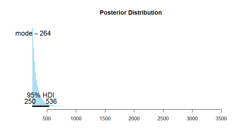
As we can see, the posterior mode is 264, not 250. The posterior mean is 336, and the median is 297. The 95% highest posterior density interval lies between 250 and 536. Therefore, the most probable total number of customers Bon Me served on that day is 264. Not so much apart from the original 250 huh? This result is based on only one sample, but if your sample more often, the results will converge to the true number of total customers.

As a side note, the original problem formulation changes if Bon Me refreshes its receipt numbers after a certain point. For example, if Bon Me receipt number reverts back to 1 after reaching number 20, then it's more difficult to estimate the total number of customers. Also if the receipt number is completely random, not sequential and ordered, then it's nearly impossible.