Part-of-Speech Tagging with Trigram Hidden Markov Models and the Viterbi Algorithm
Posted on June 07 2017 in Natural Language Processing
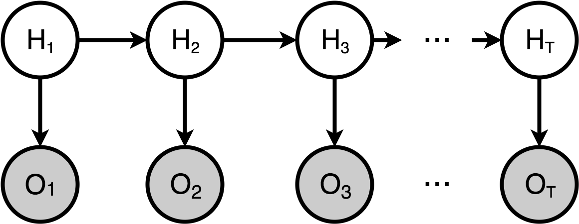
Hidden Markov Model
The hidden Markov model or HMM for short is a probabilistic sequence model that assigns a label to each unit in a sequence of observations. The model computes a probability distribution over possible sequences of labels and chooses the best label sequence that maximizes the probability of generating the observed sequence. The HMM is widely used in natural language processing since language consists of sequences at many levels such as sentences, phrases, words, or even characters.
This post presents the application of hidden Markov models to a classic problem in natural language processing called part-of-speech tagging, explains the key algorithm behind a trigram HMM tagger, and evaluates various trigram HMM-based taggers on the subset of a large real-world corpus.
Part of Speech Tagging
Part-of-speech tagging or POS tagging is the process of assigning a part-of-speech marker to each word in an input text. Tags are not only applied to words, but also punctuations as well, so we often tokenize the input text as part of the preprocessing step, separating out non-words like commas and quotation marks from words as well as disambiguating end-of-sentence punctuations such as period and exclamation point from part-of-word punctuation in the case of abbreviations like i.e. and decimals.
POS tagging is extremely useful in text-to-speech; for example, the word read can be read in two different ways depending on its part-of-speech in a sentence. A tagging algorithm receives as input a sequence of words and a set of all different tags that a word can take and outputs a sequence of tags. The algorithm works to resolve ambiguities of choosing the proper tag that best represents the syntax and the semantics of the sentence. When someone says I just remembered that I forgot to bring my phone, the word that grammatically works as a complementizer that connects two sentences into one, whereas in the following sentence, Does that make you feel sad, the same word that works as a determiner just like the, a, and an. Designing a highly accurate POS tagger is a must so as to avoid assigning a wrong tag to such potentially ambiguous word since then it becomes difficult to solve more sophisticated problems in natural language processing ranging from named-entity recognition and question-answering that build upon POS tagging.
The Brown Corpus
In the following sections, we are going to build a trigram HMM POS tagger and evaluate it on a real-world text called the Brown corpus which is a million word sample from 500 texts in different genres published in 1961 in the United States. We train the trigram HMM POS tagger on the subset of the Brown corpus containing nearly 27500 tagged sentences in the development test set, or devset Brown_dev.txt. The accuracy of the tagger is measured by comparing the predicted tags with the true tags in Brown_tagged_dev.txt. The algorithm of tagging each word token in the devset to the tag it occurred the most often in the training set Most Frequenct Tag is the baseline against which the performances of various trigram HMM taggers are measured.
It is useful to know as a reference how the part-of-speech tags are abbreviated, and the following table lists out few important part-of-speech tags and their corresponding descriptions.
| Tag | Description | Example |
|---|---|---|
| IN | Preposition | in, by, of |
| JJ | Adjective | green, happy |
| NN | Singular Noun | paper, word |
| NNS | Plural Noun | papers, words |
| PRP | Personal Pronoun | you, he, she |
| VB | Verb Base Form | take, eat, run |
| VBD | Verb Past Tense | took, ate, ran |
| . | Sentence-Final Punctuation | . ! ? |
Here is an example sentence from the Brown training corpus.
At/ADP that/DET time/NOUN highway/NOUN engineers/NOUN traveled/VERB
rough/ADJ and/CONJ dirty/ADJ roads/NOUN to/PRT accomplish/VERB their/DET duties/NOUN ./.
Each sentence is a string of space separated WORD/TAG tokens, with a newline character in the end. Notice how the Brown training corpus uses a slightly different notation than the standard part-of-speech notation in the table above. Let's now discuss the method for building a trigram HMM POS tagger.
Trigram HMM Part-of-Speech Tagger
Decoding is the task of determining which sequence of variables is the underlying source of some sequence of observations. Mathematically, we want to find the most probable sequence of hidden states \(Q = q_1,q_2,q_3,...,q_N\) given as input a HMM \(\lambda = (A,B)\) and a sequence of observations \(O = o_1,o_2,o_3,...,o_N\) where \(A\) is a transition probability matrix, each element \(a_{ij}\) represents the probability of moving from a hidden state \(q_i\) to another \(q_j\) such that \(\sum_{j=1}^{n} a_{ij} = 1\) for \(\forall i\) and \(B\) a matrix of emission probabilities, each element representing the probability of an observation state \(o_i\) being generated from a hidden state \(q_i\). In POS tagging, each hidden state corresponds to a single tag, and each observation state a word in a given sentence. For example, the task of the decoder is to find the best hidden tag sequence DT NNS VB that maximizes the probability of the observed sequence of words The dogs run.
Define \(\hat{q}_{1}^{n} = \hat{q}_1,\hat{q}_2,\hat{q}_3,...,\hat{q}_n\) to be the most probable tag sequence given the observed sequence of \(n\) words \(o_{1}^{n} = o_1,o_2,o_3,...,o_n\). Then we have the decoding task:
where the second equality is computed using Bayes' rule. Moreover, the denominator \(P(o_{1}^{n})\) can be dropped in Eq. 1 since it does not depend on \(q_{1}^{n}\).
where \(P(q_{1}^{n})\) is the probability of a tag sequence, \(P(o_{1}^{n} \mid q_{1}^{n})\) is the probability of the observed sequence of words given the tag sequence, and \(P(o_{1}^{n}, q_{1}^{n})\) is the joint probabilty of the tag and the word sequence. The trigram HMM tagger makes two assumptions to simplify the computation of \(P(q_{1}^{n})\) and \(P(o_{1}^{n} \mid q_{1}^{n})\). The first is that the emission probability of a word appearing depends only on its own tag and is independent of neighboring words and tags:
The second is a Markov assumption that the transition probability of a tag is dependent only on the previous two tags rather than the entire tag sequence:
where \(q_{-1} = q_{-2} = *\) is the special start symbol appended to the beginning of every tag sequence and \(q_{n+1} = STOP\) is the unique stop symbol marked at the end of every tag sequence.
In many cases, we have a labeled corpus of sentences paired with the correct POS tag sequences The/DT dogs/NNS run/VB such as the Brown corpus, so the problem of POS tagging is that of the supervised learning where we easily calculate the maximum likelihood estimate of a transition probability \(P(q_i \mid q_{i-1}, q_{i-2})\) by counting how often we see the third tag \(q_{i}\) followed by its previous two tags \(q_{i-1}\) and \(q_{i-2}\) divided by the number of occurrences of the two tags \(q_{i-1}\) and \(q_{i-2}\):
Similarly we compute an emission probability \(P(o_i \mid q_i)\) as follows:
The Viterbi Algorithm
Recall that the decoding task is to find
where the argmax is taken over all sequences \(q_{1}^{n}\) such that \(q_i \in S\) for \(i=1,...,n\) and \(S\) is the set of all tags. We further assume that \(P(o_{1}^{n}, q_{1}^{n})\) takes the form
assuming \(q_{-1} = q_{-2} = *\) and \(q_{n+1} = STOP\). Because the argmax is taken over all different tag sequences, brute force search where we compute the likelihood of the observation sequence given each possible hidden state sequence is hopelessly inefficient as it is \(O(|S|^3)\) in complexity. Instead, the Viterbi algorithm, a kind of dynamic programming algorithm, is used to make the search computationally more efficient.
Define \(n\) to be the length of the input sentence and \(S_k\) for \(k = -1,0,...,n\) to be the set of possible tags at position k such that \(S_{-1} = S_0 = {*}\) and \(S_k = S k \in {1,...,n}\). Define
and a dynamic programming table, or a cell, to be
which is the maximum probability of a tag sequence ending in tags \(u\), \(v\) at position \(k\). The Viterbi algorithm fills each cell recursively such that the most probable of the extensions of the paths that lead to the current cell at time \(k\) given that we had already computed the probability of being in every state at time \(k-1\). In a nutshell, the algorithm works by initializing the first cell as
and for any \(k \in {1,...,n}\), for any \(u \in S_{k-1}\) and \(v \in S_k\), recursively compute
and return
The last component of the Viterbi algorithm is backpointers. The goal of the decoder is to not only produce a probability of the most probable tag sequence but also the resulting tag sequence itself. The best state sequence is computed by keeping track of the path of hidden state that led to each state and backtracing the best path in reverse from the end to the start. A full implementation of the Viterbi algorithm is shown.
from collections import defaultdict, deque

START_SYMBOL = '*'
STOP_SYMBOL = 'STOP'
LOG_PROB_OF_ZERO = -1000

def viterbi(brown_dev_words, taglist, known_words, q_values, e_values):
    # pi[(k, u, v)]: max probability of a tag sequence ending in tags u, v
    # at position k
    # bp[(k, u, v)]: backpointers to recover the argmax of pi[(k, u, v)]
    tagged = []
    pi = defaultdict(float)
    bp = {}

    # Initialization
    pi[(0, START_SYMBOL, START_SYMBOL)] = 0.0

    # Define tagsets S(k)
    def S(k):
        if k in (-1, 0):
            return {START_SYMBOL}
        else:
            return taglist

    # The Viterbi algorithm
    for sent_words_actual in brown_dev_words:
        sent_words = [word if word in known_words else subcategorize(word) \
                      for word in sent_words_actual]
        n = len(sent_words)
        for k in range(1, n+1):
            for u in S(k-1):
                for v in S(k):
                    max_score = float('-Inf')
                    max_tag = None
                    for w in S(k - 2):
                        if e_values.get((sent_words[k-1], v), 0) != 0:
                            score = pi.get((k-1, w, u), LOG_PROB_OF_ZERO) + \
                                    q_values.get((w, u, v), LOG_PROB_OF_ZERO) + \
                                    e_values.get((sent_words[k-1], v))
                            if score > max_score:
                                max_score = score
                                max_tag = w
                    pi[(k, u, v)] = max_score
                    bp[(k, u, v)] = max_tag

        max_score = float('-Inf')
        u_max, v_max = None, None
        for u in S(n-1):
            for v in S(n):
                score = pi.get((n, u, v), LOG_PROB_OF_ZERO) + \
                        q_values.get((u, v, STOP_SYMBOL), LOG_PROB_OF_ZERO)
                if score > max_score:
                    max_score = score
                    u_max = u
                    v_max = v

        tags = deque()
        tags.append(v_max)
        tags.append(u_max)

        for i, k in enumerate(range(n-2, 0, -1)):
            tags.append(bp[(k+2, tags[i+1], tags[i])])
        tags.reverse()

        tagged_sentence = deque()
        for j in range(0, n):
            tagged_sentence.append(sent_words_actual[j] + '/' + tags[j])
        tagged_sentence.append('\n')
        tagged.append(' '.join(tagged_sentence))

    return tagged
Note that the function takes in data to tag brown_dev_words, a set of all possible tags taglist, and a set of all known words known_words, trigram probabilities q_values, and emission probabilities e_values, and outputs a list where every element is a tagged sentence in the WORD/TAG format, separated by spaces with a newline character in the end, just like the input tagged data. Please refer to the full Python codes attached in a separate file for more details.
Deleted Interpolation
Previously, a transition probability is calculated with Eq. 5. However, many times these counts will return a zero in a training corpus which erroneously predicts that a given tag sequence will never occur at all. A common, effective remedy to this zero division error is to estimate a trigram transition probability by aggregating weaker, yet more robust estimators such as a bigram and a unigram probability. For instance, assume we have never seen the tag sequence DT NNS VB in a training corpus, so the trigram transition probability \(P(VB \mid DT, NNS) = 0\) but it may still be possible to compute the bigram transition probability \(P(VB | NNS)\) as well as the unigram probability \(P(VB)\).
More generally, the maximum likelihood estimates of the following transition probabilities can be computed using counts from a training corpus and subsequenty setting them to zero if the denominator happens to be zero:
where \(N\) is the total number of tokens, not unique words, in the training corpus. The final trigram probability estimate \(\tilde{P}(q_i \mid q_{i-1}, q_{i-2})\) is calculated by a weighted sum of the trigram, bigram, and unigram probability estimates above:
under the constraint \(\lambda_{1} + \lambda_{2} + \lambda_{3} = 1\). These values of \(\lambda\)s are generally set using the algorithm called deleted interpolation which is conceptually similar to leave-one-out cross-validation LOOCV in that each trigram is successively deleted from the training corpus and the \(\lambda\)s are chosen to maximize the likelihood of the rest of the corpus. The deletion mechanism thereby helps set the \(\lambda\)s so as to not overfit the training corpus and aid in generalization. The Python function that implements the deleted interpolation algorithm for tag trigrams is shown.
import numpy as np
from collections import defaultdict

def deleted_interpolation(unigram_c, bigram_c, trigram_c):
    lambda1 = lambda2 = lambda3 = 0
    for a, b, c in trigram_c.keys():
        v = trigram_c[(a, b, c)]
        if v > 0:
            try:
                c1 = float(v-1)/(bigram_c[(a, b)]-1)
            except ZeroDivisionError:
                c1 = 0
            try:
                c2 = float(bigram_c[(a, b)]-1)/(unigram_c[(a,)]-1)
            except ZeroDivisionError:
                c2 = 0
            try:
                c3 = float(unigram_c[(a,)]-1)/(sum(unigram_c.values())-1)
            except ZeroDivisionError:
                c3 = 0

            k = np.argmax([c1, c2, c3])
            if k == 0:
                lambda3 += v
            if k == 1:
                lambda2 += v
            if k == 2:
                lambda1 += v

    weights = [lambda1, lambda2, lambda3]
    norm_w = [float(a)/sum(weights) for a in weights]
    return norm_w
Note that the inputs are the Python dictionaries of unigram, bigram, and trigram counts, respectively, where the keys are the tuples that represent the tag trigram, and the values are the counts of the tag trigram in the training corpus. The function returns the normalized values of \(\lambda\)s.
Unknown Words
In all languages, new words and jargons such as acronyms and proper names are constantly being coined and added to a dictionary. Keep updating the dictionary of vocabularies is, however, too cumbersome and takes too much human effort. Thus, it is important to have a good model for dealing with unknown words to achieve a high accuracy with a trigram HMM POS tagger.
RARE
RARE is a simple way to replace every word or token with the special symbol _RARE_ whose frequency of appearance in the training set is less than or equal to 5. Without this process, words like person names and places that do not appear in the training set but are seen in the test set can have their maximum likelihood estimates of \(P(q_i \mid o_i)\) undefined.
MORPHO
MORPHO is a modification of RARE that serves as a better alternative in that every word token whose frequency is less than or equal to 5 in the training set is replaced by further subcategorization based on a set of morphological cues. For example, we all know that a word with suffix like -ion, -ment, -ence, and -ness, to name a few, will be a noun, and an adjective has a prefix like un- and in- or a suffix like -ious and -ble. Take a look at the following Python function.
import re

RARE_SYMBOL = '_RARE_'
RARE_WORD_MAX_FREQ = 5

def subcategorize(word):
    if not re.search(r'\w', word):
        return '_PUNCS_'
    elif re.search(r'[A-Z]', word):
        return '_CAPITAL_'
    elif re.search(r'\d', word):
        return '_NUM_'
    elif re.search(r'(ion\b|ty\b|ics\b|ment\b|ence\b|ance\b|ness\b|ist\b|ism\b)',word):
        return '_NOUNLIKE_'
    elif re.search(r'(ate\b|fy\b|ize\b|\ben|\bem)', word):
        return '_VERBLIKE_'
    elif re.search(r'(\bun|\bin|ble\b|ry\b|ish\b|ious\b|ical\b|\bnon)',word):
        return '_ADJLIKE_'
    else:
        return RARE_SYMBOL
Results
The most frequent tag baseline Most Frequent Tag where every word is tagged with its most frequent tag and the unknown or rare words are tagged as nouns by default already produces high tag accuracy of around 90%. The tag accuracy is defined as the percentage of words or tokens correctly tagged and implemented in the file POS-S.py in my github repository. This is partly because many words are unambiguous and we get points for determiners like the and a and for punctuation marks. The average run time for a trigram HMM tagger is between 350 to 400 seconds. The weights \(\lambda_1\), \(\lambda_2\), and \(\lambda_3\) from deleted interpolation are 0.125, 0.394, and 0.481, respectively.
Most Frequent Tag:90%Trigram HMM Viterbi (+ Deleted Interpolation + RARE):91.15%Trigram HMM Viterbi (+ Deleted Interpolation + MORPHO):92.18%Trigram HMM Viterbi (- Deleted Interpolation + RARE):93.32%Trigram HMM Viterbi (- Deleted Interpolation + MORPHO):94.25%Upper Bound (Human Agreement):98%
The trigram HMM tagger with no deleted interpolation and with MORPHO results in the highest overall accuracy of 94.25% but still well below the human agreement upper bound of 98%. Such 4 percentage point increase in accuracy from the most frequent tag baseline is quite significant in that it translates to \(10000 \times 0.04 = 400\) additional sentences accurately tagged. Also note that using the weights from deleted interpolation to calculate trigram tag probabilities has an adverse effect in overall accuracy. This is most likely because many trigrams found in the training set are also found in the devset, rendering useless bigram and unigram tag probabilities.
In this post, we introduced the application of hidden Markov models to a well-known problem in natural language processing called part-of-speech tagging, explained the Viterbi algorithm that reduces the time complexity of the trigram HMM tagger, and evaluated different trigram HMM-based taggers with deleted interpolation and unknown word treatments on the subset of the Brown corpus. The result is quite promising with over 4 percentage point increase from the most frequent tag baseline but can still be improved comparing with the human agreement upper bound. The hidden Markov models are intuitive, yet powerful enough to uncover hidden states based on the observed sequences, and they form the backbone of more complex algorithms.
You can find all of my Python codes and datasets in my Github repository here!