Predicting the Fitbit Challenge Winner with Hierarchical Bayes
Posted on November 28 2015 in Bayesian Statistics
Hi there! It's been a little more than a month since my last post. Thanksgiving was two days ago, and I had a good time with my family. How's everyone doing?
With the upcoming Cyber Monday, I'm sure many of you have cool electronics and gadgets in mind to look forward to buying. One of my recommendations is Fitbit, which is a health and fitness wearable that keeps track of daily activities and workouts. I bought a Charge HR, one of many Fitbit products for active fitness, not too long ago because I thought I'd get more motivated to exercise regularly and lose weight if I wore it on my wrist all the time. How do I feel about it so far? I really like it! While wearing, it counts my steps, estimates calories lost, and even tracks my heartbeat in real-time. Every night I come home and sync data with the Fitbit app in my phone via Bluetooth and feel good about my exercise and workout achievements. I've also recently started competing against two of my friends in a Fitbit weekly challenge where a person with the greatest total number of steps taken during the workweek wins the challenge. We've decided to make it more interesting by having the second and the last place pay for snacks every Sunday night after the challenge with the second place responsible for \(1/3\) and the last \(2/3\) of the expense. So far, I've been the last place for four times in a row which is a bit discouraging but nonetheless incentivizes me to aim for the first place by walking and running more. I have my own "excuses" for that, but that's not the focus of this post so I won't get into the details.
the data
The main focus of this post, then, is that I want to be able to predict who's going to win the weekly challenge for the next week using data from the past weeks. But I realized that Fitbit doesn't store all the weekly challenge data forever, so I was only able to retrieve data for the past three weeks including this week. For example, A came in first two weeks ago with about 53K steps total, B took about 36K steps coming in second, and person C was the last place with a little more than 24K steps. The dataset from the challenge looks like the following:
| Participant ID | Steps | Max Date |
|---|---|---|
| A | 53497 | 2015-11-13 |
| A | 51667 | 2015-11-20 |
| A | 39039 | 2015-11-27 |
| B | 36315 | 2015-11-13 |
| B | 27629 | 2015-11-20 |
| B | 46166 | 2015-11-27 |
| C | 24256 | 2015-11-13 |
| C | 19076 | 2015-11-20 |
| C | 37665 | 2015-11-27 |
where the column max date is the last date of a weekly challenge which is Friday and the actual participant names are replaced by the alphabetical ids. The question is whether the variation in the number of steps within each subject can be used to predict the steps for each subject for the next week with the max date 2015-12-04 from which I calculate each subject's probability of being the first, second and last place. I'm going to assume that each subject or participant is independent of the others in steps; for instance, the number of steps taken by A for the past three weeks has nothing to do with the number of steps by B and C during the same time frame. Statistically speaking, this means the number of steps are drawn from A's true, innate step distribution only. Though I see that the steps taken by A, B, and C respectively are generally higher for the past weeks, the data is small enough to lack a clear justification for such trend and possible correlation among participants.
the methods
An easy way to solve this problem is to use a Bayesian linear mixed model by setting the participant ids as the random effect to predict the number of steps. But this formulation is too limiting in that I assume each participant's steps to be normally distributed which may not be the case.
Instead, I'm going to construct a full hierarchical Bayesian model in JAGS, which stands for Just Another Gibbs Sampler that analyzes it using Markov Chain Monte Carlo (MCMC) simulation, that captures the variability of steps within subject as well as my prior knowledge of each subject's weekly step tendency. Here we have a probabilistic generative model for each participant:
where
\(\theta\) and \(\omega\) represent the mean and the standard deviation respectively which are the reparameterization of \(\alpha\) the shape parameter and \(\beta\) the rate parameter for the purpose of convenience. Often it's far more intuitive to work with the mean and the standard deviation because we think in terms of central tendency and deviation away from the center than rather obscure shape and rate parameters. For each subject, I've assumed his or her steps \(y_i\) to be independently and identically Gamma distributed with non-zero mode instead of the traditional normal distribution because steps can't be negative and the Gamma distribution accounts for the long tail in steps that goes beyond the average number of steps taken by the subject. The prior distribution for \(\theta\) is normal at mean \(\mu\) and standard deviation \(\sigma\) where I'm going to set \(\mu\) to be the subject-level mean and \(\sigma\) to be wide in the range of data for all subjects. The uninformative prior for \(\omega\) is a uniform distribution with the minimum at \(L\) and the maximum at \(H\) both of which are also set to be wide in the range of data that accounts for all possible variability in steps. The diagram below shows the equations above in a hierarchical structure:
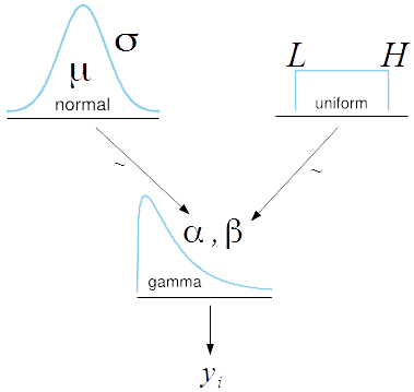
The following is the equivalent JAGS syntax. As you can see, \(yMean\) represents a subject-level mean and \(ySD\) the standard deviation of the steps for all subjects. So here I'm saying that \(\omega\), the standard deviation of the steps for each subject, can range from anywhere between \(\frac{ySD}{100}\) and \(ySD \times 10\) which scales quite extensive. In addition, the standard deviation \(\sigma\) of the normally distributed random variable \(\theta\) is \((ySD \times 10)^2\) which is also wide in the range of data but is actually written as \(\frac{1}{(ySD \times 10)^2}\) since JAGS works with the precision values.
model {
    for (i in 1:N) {
        y[i] ~ dgamma(alpha, beta)
    }
    alpha <- pow(theta, 2) / pow(omega, 2)
    beta <- theta / pow(omega, 2)
    theta ~ dnorm(yMean, 1/(ySD*10)^2)
    omega ~ dunif(ySD/100, ySD*10)
}
A full hierarchical Bayesian model like this is intuitive, yet powerful in that the posterior estimates and their uncertainties are robust and reflective of prior information on the challenge participants.
the distributions
After running three separate sets of MCMC simulations, one set of \(50000\) simulations per subject, I get the posterior predictive distribution of the average number of steps for A that looks like this:
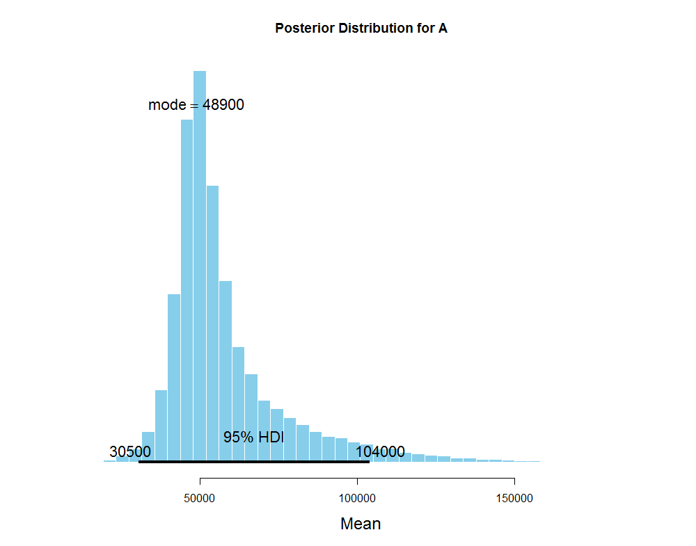
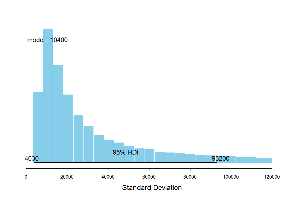
The average number of steps for A has the 95% highest posterior density interval between 31K and 117K steps. Since the resulting posterior distribution is skewed, it's better to use the mode which is 52.7K to describe the central tendency of the average number of steps instead of the mean. The posterior predictive distribution of the standard deviation of steps for A:
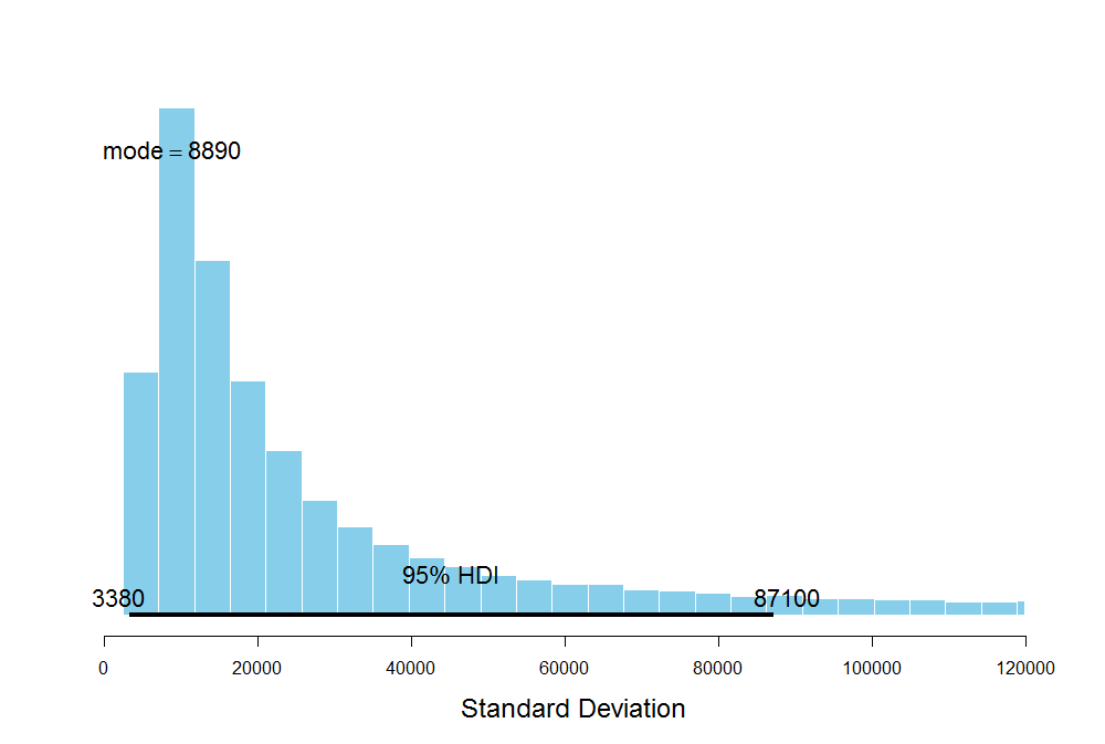
The 95% credibility interval for the standard deviation of steps is quite large which is plausible since I don't have much data at hand to be very certain about my estimates of the average number of steps for A. This is also the result of using the uninformative prior for \(\omega\), representing the subject-level standard deviation of steps, where the prior seems to dominate the likelihood due to high uncertainty from the lack of data itself. Similarly, these are the results for B and C:
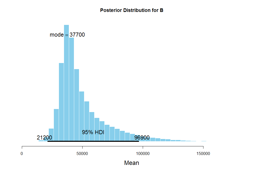
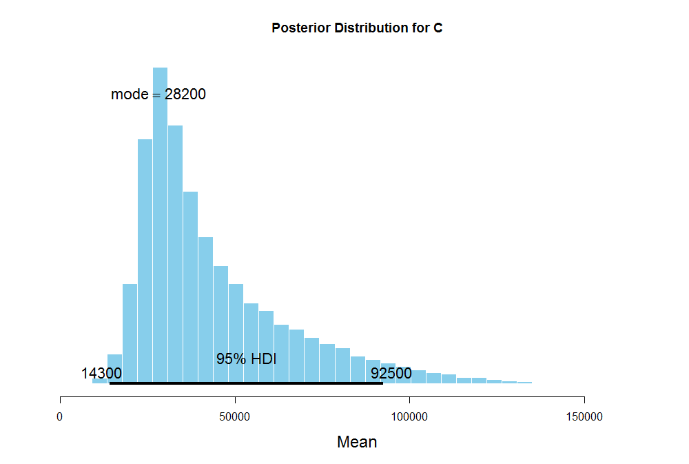
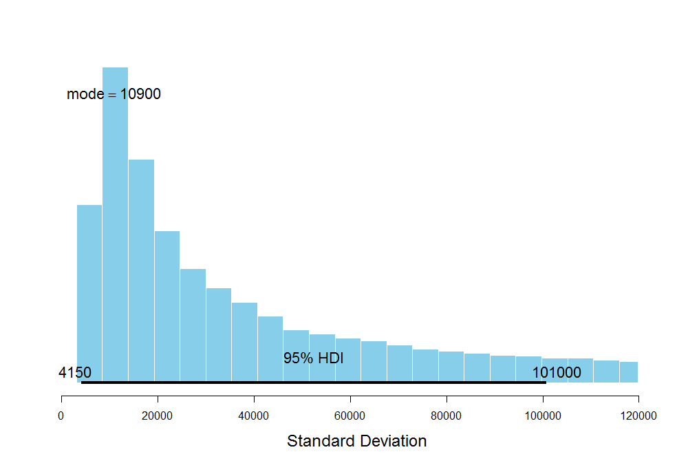
The mode of the average number of steps for B is about 37.4K with the standard deviation ranging from 4K to 95K which also signifies a large uncertainty in our estimates of the average steps. The mode for C is 28.5K which is way below 37.4K steps for B, but its uncertainty is huge as well.
Next I'm going to use these posterior distributions of the mean number of steps for A, B, and C to calculate the probability of placing first, second, and last for each participant in the challenge next week.
the predictions
The MCMC simulations for the three participants return \(50000\) sample steps from their respective posterior predictive distributions. Using those \(50000\) sample steps for each subject, I can order three participants in decreasing order, creating the columns first, second, and last:
| Observation | A | B | C | First | Second | Last |
|---|---|---|---|---|---|---|
| 1 | 50237 | 34798 | 25127 | A | B | C |
| 2 | 53579 | 44662 | 40684 | A | B | C |
| 3 | 48365 | 37662 | 42237 | A | C | B |
| 4 | 48806 | 41669 | 57515 | C | A | B |
| 5 | 39237 | 31379 | 48063 | C | A | B |
| ... | ... | ... | ... | ... | ... | ... |
Now I can calculate how many times out of \(50000\) sample observations did A, B, and C win first, second, and last place. The table below writes the probability of each place for every subject:
| Participant ID | P(First) | P(Second) | P(Last) |
|---|---|---|---|
| A | 0.5328 | 0.3606 | 0.1066 |
| B | 0.2591 | 0.4195 | 0.3214 |
| C | 0.2081 | 0.2199 | 0.5720 |
Therefore, A has 53% chance of winning next week, while B has approximately 26% chance of achieving the first place and C only 21% chance. These estimates are very different from the common frequentist estimates of \(2/3\), or 67%, naively calculated from A's past 2 wins out of 3 total. Also if the steps in each week is independent of that in the other weeks, like a coin toss, then the probability of winning for A, B, and C is all equivalent to \(1/3\), or 33%.
When I actually ran the analysis, I also computed how much money A, B, and C are going to lose by the end of 3 months using a Monte Carlo simulation from the triangular distribution. I won't discuss the details here, but the results were that A is likely to lose about $71, B $79, and C $134. Interesting!
I've formulated a hierarchical Bayesian model in JAGS in R to predict the probability of winning for A, B, and C which is more realistic, intuitive, and robust than the usual naive frequentist approach. Hope this was a fun read for you! Let me know if you have any questions or suggestions.